Mechanistic Interpretability
What is Mechanistic Interpretability and why do we care ?
Neural Networks are just an advanced mapping from input to output in other words it is a way to find the approximate function that will produce the correct output based on the input.
As we know functions may have many paramters and understanding those paramters is not usually intuitive and the same thing for nuerons in neural networks.
The process of reverse-engineering the functionality of those parameters is called Mechanistic Interpretability.
Here we are going to talk about the interpretability of Attention based Large Langauge Models but it is worth noting that this field goes beyond that.
It's critically useful to understand how a model is working for showing:
- Is the model generalizing or just memorizing?
- Are its internal objectives aligned with its intended goals?
For example, Anthropic found that a model can explicitly misstate its own reasoning process, describing its approach in a way that doesn't reflect what it's actually doing.[1]
By reverse-engineering what works in existing networks, we can distill principles for next-generation designs
In this post we are trying to reproduce the results of 2 main papers by Anthropic[2, 3]
Transformers & Attention
If you haven't been living under a rock you probably have heard about Transformers[4], in which they introduced the Multi head attention (MHA) the most important part today.
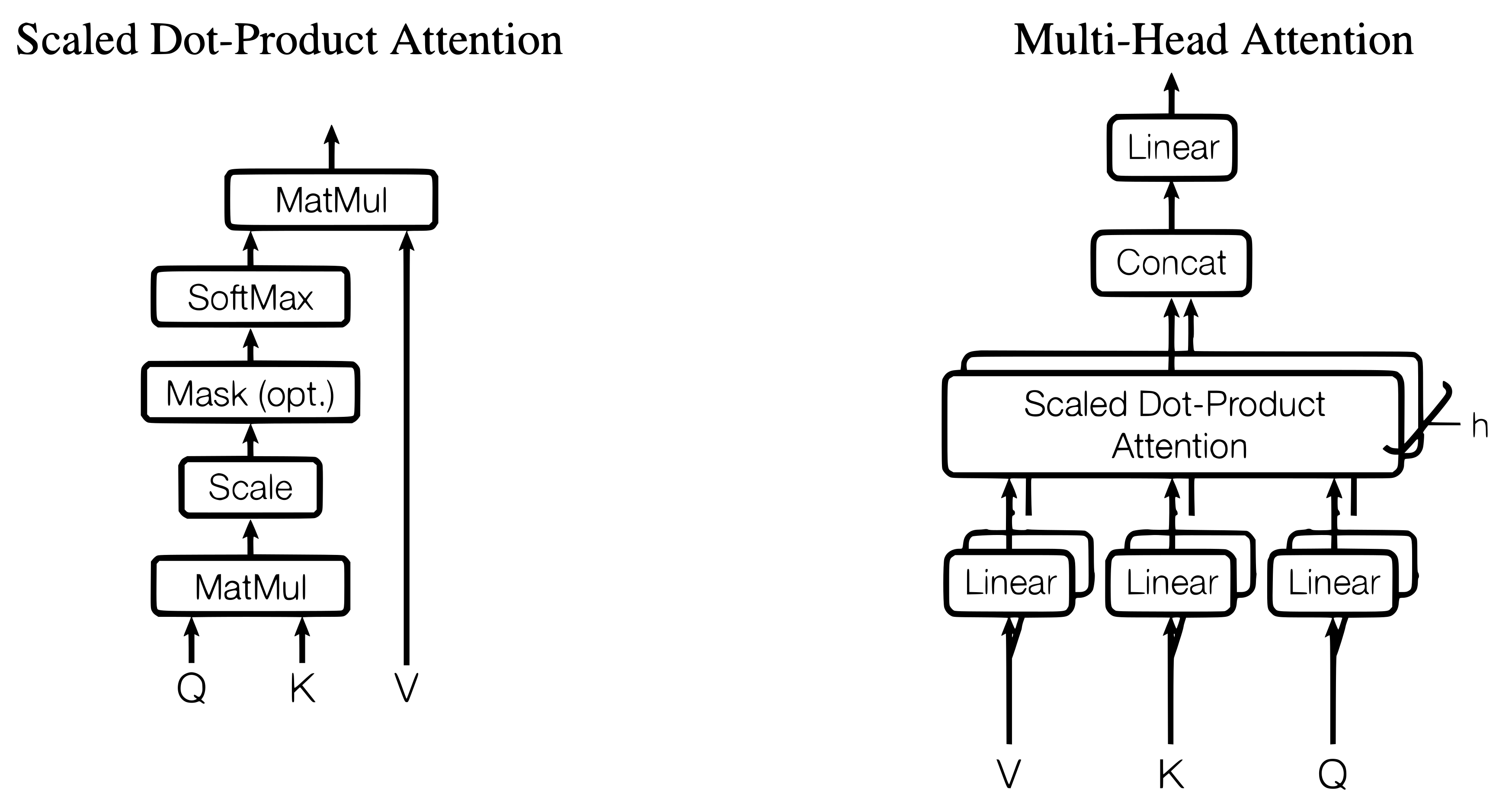
Eventhough the architecture have changed a little bit for optimization purposes and many varations have been introduced (GQA, MLA, DSA ...) still they all are some few tweaks away from original.
Almost all of the performance gained by LLMs are because of this part that's why we are going to focus on it solely, meaning we will be training and inspecting Attention-only models ranging from 1, 2, 3 and 8 layers in the first few experiments and then migrate to analyze a model like gpt2.
NOTE: We are not using MLPs here because they famously make models hard to interpret due to their tendency to create distributed representations.
One-Layer Transformer
Starting we are training our model on openwebtext dataset, using a One-Layer attention only transformer
using the following paramters:
enc = tiktoken.get_encoding("gpt2")
d_model = 768
n_heads = 12
d_head = 64
vocab_size = enc.n_vocab
batch_size = 32
context_len = 128
lr = 3e-4
epochs = 40_000
eval_iters = 50Training a single layer with 12 heads and a context of 128 tokens.
class OneLayerTransformer(nn.Module):
    def __init__(self, vocab_size: int, d_model: int, n_heads: int, d_head: int, context_len: int):
        super().__init__()
        self.vocab_size = vocab_size
        self.d_model = d_model
        self.n_heads = n_heads
        self.d_head = d_head
        self.context_len = context_len
        # Embedding
        self.W_E = nn.Embedding(self.vocab_size, self.d_model)
        self.W_pos = nn.Embedding(context_len, d_model)
        self.W_Q = nn.Linear(self.d_model, self.n_heads * self.d_head, bias=False)
        self.W_K = nn.Linear(self.d_model, self.n_heads * self.d_head, bias=False)
        self.W_V = nn.Linear(self.d_model, self.n_heads * self.d_head, bias=False)
        self.W_O = nn.Linear(self.n_heads * self.d_head, self.d_model, bias=False)
        # Unembedding
        self.W_U = nn.Linear(self.d_model, self.vocab_size)

    def forward(self, x: torch.Tensor, return_all: bool = False) -> torch.Tensor:
        device = x.device
        d_head, n_heads = self.d_head, self.n_heads
        B, T = x.shape
        pos = torch.arange(T, device=device)
        x = self.W_E(x) + self.W_pos(pos)

        residual = x
        # B, T, C
        q = self.W_Q(x) # (B, T, n_heads * d_head)
        k = self.W_K(x)
        v = self.W_V(x)

        # To parallelize acros heads and batches
        q = q.view(B, T, n_heads, d_head).transpose(1, 2)
        v = v.view(B, T, n_heads, d_head).transpose(1, 2)
        k = k.view(B, T, n_heads, d_head).transpose(1, 2)
                                # B, T, n_heads, d_head -> B, T, n_heads, d_head
        scores = torch.matmul(q, k.transpose(-2, -1)) / d_head ** 0.5 # [B, n_heads, T, d_head] @ [B, n_heads, d_head, T] = B, n_heads, T, T
        mask = torch.triu(torch.ones(T, T, device=device, dtype=torch.bool), diagonal=1)
        scores = scores.masked_fill(mask, float('-inf'))
        # 4. Softmax
        pattern = F.softmax(scores, dim=-1)

        z = torch.matmul(pattern, v) # [B, n_heads, T, d_head]
        z = z.transpose(1, 2).contiguous().view(B, T, -1)
        attn_out = self.W_O(z)

        hidden_state = attn_out + residual
        logits = self.W_U(hidden_state)
        if return_all:
            return logits, scores, pattern, v, z, hidden_state
return logits we can describe attention model as a residual stream which get branched and on that branch some filters are applied, then we add the result back onto the stream also we consider each head as its own filter and each layer as a group of filters each learning its own representation.
considering this we can also say the function of each head in attention only model is specific which means the function of a head doesn't change.
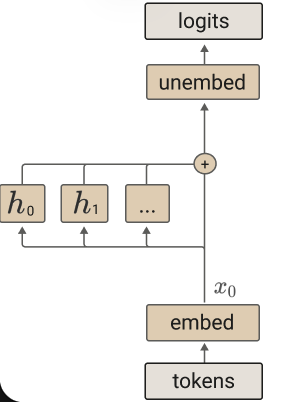
NOTE: we have to emphasize on this point because when adding MLP layer a phenomenon called polysemanticity occur this means a single neuron fires for multiple and often unrelated features at the same time for example cat and car which makes interpretation difficult.
Mathematical analysis
Here what that looks like mathmatically:
Here we recognize two paths:
Path 1: The Direct Residual Path (Bigram):
This emebedding and unembedding path which only learns a bigram representation meaning it only uses the current position. Can't look at previous words! and exactly what a zero layer model would learn
NOTE: embedding is the process of converting the discrete tokens to a continuous vector representations.
Path 2: The Attention Head Paths:
This is where context enters. and where the model starts to pay attention to even more tokens eariler in the context, and where the model learns complex represntations.
We grouped the whole layer as a path but we can also think of each head as a path of its own.
for each head:
An attention head formula is defined by four matrices:
- : The Query matrix.
- : The Key matrix
- : The Value matrix
- : The Output(or Porjection) matrix
Circuit decomposition
1. The QK Circuit (The "Where" Path)
Shows how the attention pattern determines which tokens the head looks at, meaning it filters and ranks the context (Each head has a different criteria based on which it ranks the context)
To find this, we look inside the at the term that determines the attention scores. Let be the vector at the current position (the query) and be the vector at a previous position (the key). The raw score (logit) before softmax is:
Expanding into its token embeddings :
We can group the weight matrices in the middle to find the QK Circuit:
and in the model this looks like:
@torch.no_grad()
def extract_qk_matrix(
    model: OneLayerTransformer,
    head_idx: int
) -> torch.Tensor:
    W_E = model.W_E.weight.T  # [d_model, V]
    W_Q = model.W_Q.weight  # [h*d_head, d_model]
    W_K = model.W_K.weight

    start = head_idx * d_head
    end = (head_idx + 1) * d_head

    W_Q_i = W_Q[start:end, :].T
    W_K_i = W_K[start:end, :].T
    QK = W_E.T @ W_Q_i @ W_K_i.T @ W_E
return QK2. OV Circuit (The "What" Path)
Transforms each attended token into contributions to the residual stream meaning it pushes the information based on the ranking by the QK cirucit
Both means: If QK says “B is most important token in the context” OV says “looking at B like this increases the chance of token X next.”
If we ignore the attention pattern for a moment and look at how a single vector at a source position is transformed into a contribution to the logits at the destination, we see this chain of linear transformations:
By substituting , the end-to-end linear map is:
@torch.no_grad()
def extract_ov_matrix(
    model: OneLayerTransformer,
    head_idx: int
) -> torch.Tensor:
    W_E_T = model.W_E.weight.T      # [d_model, V]
    W_U   = model.W_U.weight        # [V, d_model]

    W_V = model.W_V.weight          # [h*d_head, d_model]
    start = head_idx * d_head
    end = (head_idx + 1) * d_head
    W_V_i = W_V[start:end, :]       # [d_head, d_model]

    W_O = model.W_O.weight          # [d_model, h*d_head]
    W_O_i = W_O[:, start:end]       # [d_model, d_head]
    OV = W_U @ (W_O_i @ (W_V_i @ W_E_T))
return OVNow that we have layed the ground we can start with the analysis:
sample output:
The reality of life is vernacular or a large component by the woman.

The following the first that was no evidence in terms a “to-be.”

A couple of thousand, which will have more for the personal security for a lot of this the situation and the murder (or), a real person known to be in the past, but “histice the world.”

The next round are all the states in the case, no credit from the world’We can see from a sample output the model is outputing something that is not really understandable but we can also observer that the model is learning the structure of a language.
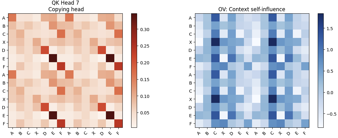
We can already see the copying mechanism here, observing the token 'E' we can see it boosting the previous token 'E'.
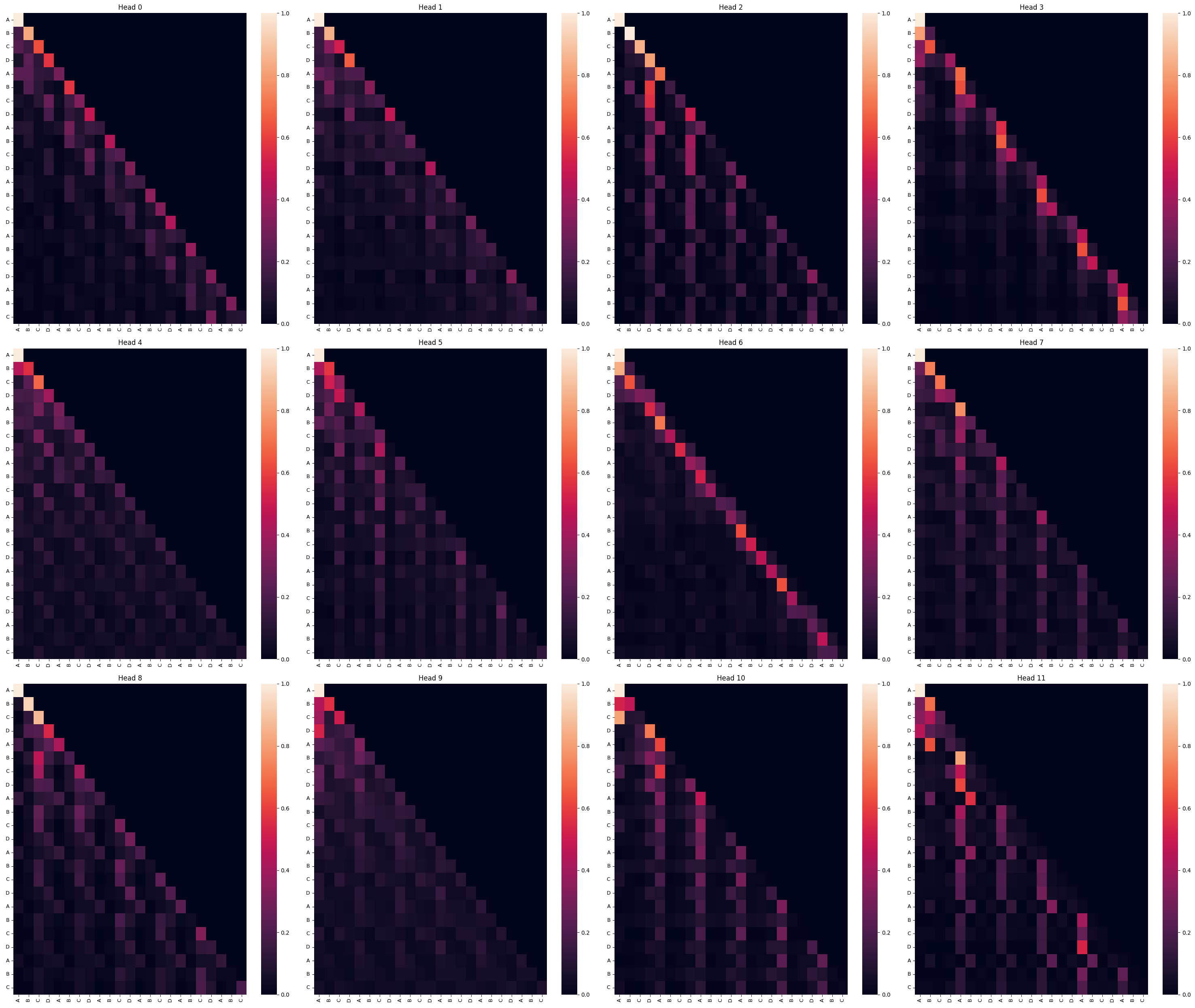
Examining the 4th, 5th and 7th heads here we can observe that those heads are doing an indication of copying and forming an early stage of what is called induction heads.
But here is the catch: copying is not the same as induction, and our one-layer model is about to walk straight into a wall.
Where one layer breaks
Let's give the model an exam. We feed it a sequence that repeats a clear pattern and ask it to continue:
A B C X D E F A B C X D E F A B C X D EThe next token should obviously be F. A human grabs it instantly: we have seen ... D E F twice already, we are sitting right after D E, so F comes next. Here is what our one-layer model thinks instead:
| Rank | Token | Probability |
|---|---|---|
| 0 | B | 2.80% |
| 1 | D | 2.79% |
| 2 | J | 2.58% |
| 3 | R | 2.25% |
| 4 | AN | 2.02% |
| ... | ... | ... |
| 25 | F | 0.70% |
F is hiding all the way down at rank 25 with a measly 0.70%. Notice the model isn't clueless, it is piling its mass on single capital letters (B, D, J, R ...), so it has clearly learned "a letter probably comes next". It just completely fails to grab the actual pattern.
Maybe that pattern was too hard? Let's make it embarrassingly easy, a pure periodic repetition:
A B C D A B C D A B C D A B C D
A B CThe continuation is just D. And still:
| Rank | Token | Probability |
|---|---|---|
| 0 | C | 1.54% |
| 1 | er | 1.51% |
| 2 | ä | 1.50% |
| 3 | L | 1.43% |
| ... | ... | ... |
| 10 | D | 1.15% |
D lands at rank 10. The model has a vague feeling that something is repeating, but it cannot commit to it.
NOTE: the token weirdness you see (AN, er, ä ...) is just the BPE tokenizer talking, single letters are rare tokens so the model smears probability over visually similar fragments.
So why does a head that provably copies still fail to predict? The answer lives in the OV circuit. Remember a head computes:
The QK circuit can make large whenever , so it reliably finds where the same token appeared before. But once it lands on that position , the OV circuit writes back a representation of itself, the very token it just matched. It is shouting "I have seen this token!", not "here is the token that came right after it".
To do induction you need to match position and then copy from position . Formally you need to learn the map . A single head can wander around the token-identity space or shift by one position, but it cannot chain both inside one matrix multiply.
One layer can ask "where have I seen this before?" — it just has no second step to answer "...and what came next?"
And this is not a bug we can train away with more epochs. It is structural. So let's give the model the one thing it is missing: depth.
Two-Layers Transformer
Adding a second attention layer changes the whole game, because now a head in layer 2 can read what a head in layer 1 wrote into the residual stream. That single fact is the entire trick:
- Layer 1 behaves like a previous-token head: it writes a token-identity-aligned signal into the stream, essentially tagging each position with "the token before me was X".
- Layer 2 becomes the induction head: it attends using that tag, and its OV circuit shifts the match forward by one position, landing on the successor token.
That is the match → shift composition the single layer could never express, now split cleanly across two layers.

We train with almost the same recipe, just a touch longer:
d_model     = 768
n_heads     = 12
d_head      = 64
context_len = 128
batch_size  = 32
lr          = 3e-4
epochs = 50_000 # OpenWebText, trained on Apple Silicon (MPS)And the model itself is just our one-layer block, stacked, with every block adding back onto the residual stream:
class TwoLayerTransformer(nn.Module):
    """Same primitives as the one-layer model, but two attention blocks
    stacked on the residual stream. Full implementation in the repo."""
    def __init__(self, vocab_size, d_model, n_heads, d_head, context_len):
        super().__init__()
        self.W_E   = nn.Embedding(vocab_size, d_model)
        self.W_pos = nn.Embedding(context_len, d_model)
        self.blocks = nn.ModuleList([
            AttentionBlock(d_model, n_heads, d_head),  # layer 1 -> previous-token head
            AttentionBlock(d_model, n_heads, d_head),  # layer 2 -> induction head
        ])
        self.W_U = nn.Linear(d_model, vocab_size)

    def forward(self, x):
        T = x.size(-1)
        x = self.W_E(x) + self.W_pos(torch.arange(T, device=x.device))
        for block in self.blocks:
            x = x + block(x)        # each block writes back to the residual stream
return self.W_U(x)Now we hand this two-layer model the exact same two exams. First the easy periodic one (target D):
| Rank | Token | Probability |
|---|---|---|
| 0 | D | 41.64% |
| 1 | E | 1.65% |
| 2 | d | 1.22% |
| 3 | ERN | 1.17% |
D rockets from rank 10 all the way to rank 0 at 41.64%. And on the harder A B C X D E F pattern (target F):
| Rank | Token | Probability |
|---|---|---|
| 0 | F | 82.92% |
| 1 | ph | 0.70% |
| 2 | S | 0.39% |
| 3 | M | 0.38% |
F goes from 0.70% buried at rank 25 to a confident 82.92% at rank 0. Same data, same tokenizer, one extra layer, an entirely different model.
This is not "a few percentage points of accuracy". It is a qualitative switch, the model went from "some letter comes next" to genuine in-context pattern matching.
Reading the heads
Numbers are satisfying, but we promised to actually reverse-engineer this, so let's look at what the heads are doing. We measure each head's attention impact, how much it actually moves the prediction, across the sequence:

Two roles already jump out. Head 2 ramps its impact up the longer a pattern has been running, it is tracking "we are currently inside a repeat". Head 3 instead spikes right at the start of a pattern, it is detecting where a repeated block begins. Put together, that is exactly the bookkeeping induction needs.
Pushing further into heads 4, 5 and 6:

The same ability gets sharper across these heads, and head 6 is plainly doing the heavy lifting, by far the largest impact on the model's pattern matching.
And if we drop down to the raw attention maps for heads 5 and 6, the smoking gun shows up:

That bright off-diagonal stripe is the fingerprint of an induction head: instead of attending to itself (the main diagonal), each position reaches back to where the pattern last repeated, a fixed offset away.
Quantifying induction
Eyeballing heatmaps is fun, but we want a number. For layer and head , the attention weights are:
where is the query–key score and the sum runs only up to (causal masking).
Raw attention can lie to us though, a head might attend hard to a position that carries almost no information. So we weight every attended position by the norm of its value vector:
Then we define an induction score that simply measures how much of that value-weighted attention lands on the off-diagonal stripe :
Any head whose score crosses a threshold (we set it at the 95th percentile of attention mass under a null model) gets flagged as an induction head. In code that whole idea is barely a few lines:
@torch.no_grad()
def induction_score(pattern, values, delta):
    # pattern: [n_heads, T, T] attention weights for one layer
    # values:  [n_heads, T, d_head] value vectors for that layer
    v_norms  = values.norm(dim=-1)                  # [n_heads, T]
    weighted = pattern * v_norms.unsqueeze(-2)      # value-weight every attended pos
    # average the off-diagonal stripe k = j - delta
    stripe = weighted.diagonal(offset=-delta, dim1=-2, dim2=-1)
return stripe.mean(dim=-1) # one score per headScaling up: GPT-2
Toy models are perfect for understanding, but the obvious question is whether any of this survives in a real model that was never built to be interpreted. So we run the same analysis on GPT-2 [5].

And there they are. In Layer 1, heads 5 and 10 show the exact two roles we assembled by hand: a previous-token head and an induction head, the same pair Wang et al. pulled out when they reverse-engineered induction in GPT-2 [6]. The mechanism we grew inside a 2-layer attention-only toy is the same mechanism a full language model discovered on its own.
The circuit we described isn't an artifact of our simplified setup, it is a fundamental piece of how transformers learn to use their context.
So what did depth actually buy us?
The picture is clean and a little surprising. Induction heads simply do not exist in the one-layer model, and they appear reliably the moment we add a second layer. It is not a smooth ramp in accuracy, it is a switch being flipped.
A single layer just does not have the computational depth to compose the QK and OV circuits into two-step reasoning. The QK circuit can detect token identity, and the OV circuit can copy token features, but without a second layer to chain these operations, the model can never pull off the "find where this token appeared, then predict what came after it" maneuver that induction demands.
This lines up beautifully with Olsson et al. [3], who found that induction heads form during training at a sharp phase transition, the very moment the loss curve takes a sudden dip. Our experiments add a structural angle to that story: the transition isn't only an accident of training dynamics, it is forced by depth. You cannot build an induction head shallower than two layers, no matter how long you train.
Where to go next
A few threads we would love to pull on:
- Watch this transition unfold during training rather than across fixed depths, and check whether it coincides with the loss drop.
- See whether the critical threshold for induction shifts with sequence length or vocabulary size.
- Bring MLPs back into the picture and study how induction interacts with polysemanticity [7], the messy, distributed representations we deliberately avoided here.
All the code, the toy models, and the GPT-2 analysis live here:
References
- [1]Lindsey, et al., "On the Biology of a Large Language Model", Transformer Circuits, 2025.
- [2]Elhage, et al., "A Mathematical Framework for Transformer Circuits", Transformer Circuits Thread, 2021.
- [3]Olsson, et al., "In-context Learning and Induction Heads", Transformer Circuits Thread, 2022.
- [4]Vaswani, Ashish, et al. "Attention is all you need." Advances in neural information processing systems 30 (2017).
- [5]Radford, et al., "Language Models are Unsupervised Multitask Learners", OpenAI, 2019.
- [6]Wang, et al., "Interpretability in the Wild: a guide to understanding induction heads in GPT-2 small", 2022.
- [7]Elhage, et al., "Toy Models of Superposition", Transformer Circuits Thread, 2022.